PATRICIA stands for Practical Algorithm To Retrieve Information Coded in Alphanumeric. It’s a binary tree (or trie as in retrieval) based search algorithm devised by D.R. Morrison eons ago (1968 to be more precise).
PATRICIA is a general algorithm for storing {key,value} pairs in a tree. PATRICIA has some very nice characteristics, namely:
- Nodes are only added to the tree when a bit position in the key of 2 nodes differs, thus keeping the tree small and speeding up lookups
- Only 1 type of node required thus simplifying implementation (no external nodes as in radix search trees)
I do not want to delve into the details of PATRICIA here, these can be gleaned from numerous books or web pages (e.g. Robert Sedgewick’s “Algorighms in C++” or Wikipedia). However, to demonstrate how PATRICIA works, particularly when used for IP route lookups, I programmed this little simulator (to download save target as…). The PATRICIA tree simulation shows how the search tree is built up and how searches iterate through the tree nodes.
How to use the PATRICIA search tree simulator
To run the PATRICIA tree simulator, install Java 1.6 and optionally JMF (Java Media Framework) for creating JPEG images and movies of the animation. You know where you get these things.
The left hand side of the GUI contains the control elements:
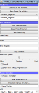
PATRICIA tree simulator controls
Control elements:
- Load Route File from Disk…: Select a route file from disk (details see below)
- Save Route File to Disk…: Save a selected route file to disk for modifications
- Drop-down box with built-in route files
- Build Tree Animation: Start animating the build-up of the tree
- Search Tree Animation: Start animating searching the tree for keys (if the Search Key field is empty, all keys of the built-in route file are searched)
- Clear Search Key: Clear Search Key, Mask and Info fields
- Search Key, Mask and Info (target) fields: Show key, mask and info encountered during search
- Stop Animation: Stop a running animation
- Animation Speed: Well, speed of the animation
- Sound!: Emit a beep for each node traversed in the search key animation
- Show Node Info …: Show node detail information during the search key animation
- Finally controls for saving the current screen as a JPEG file or saving the entire animation as a movie (uses JMF)
To run the PATRICIA tree animation, first load a route file from disk or select one of the built-in route files. Then press the Build Tree Animation button to start the animation of the build-up of the tree. Change the animation speed to your needs.
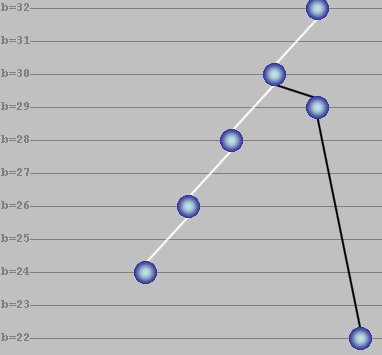
The tree is built in the draw panel with horizontal lines indicating the bit position in the key that the PATRICIA algorithm evaluates:
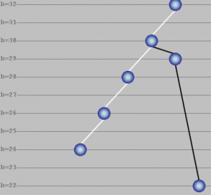
PATRICIA tree view
The blue balls represent PATRICIA tree nodes, connected to other nodes with left and right “pointers” indicated with white and black lines.
The horizontal lines indicate the bit position for which a node was inserted by the PATRICIA algorithm. In the picture above, nodes have been inserted at positions 30, 29, 28, 26, 24 and 22 (see bit position on the left hand side). The node Western union money transfer at bit position b=32 is the head node (tree root node) th Western union money transfer at is always cre Western union money transfer at ed irrespective of the route file chosen.
The tree and sub-trees can be collapsed and expanded by double-clicking a node. A collapsed sub-tree is indicated with a green ball.
PATRICIA tree node information
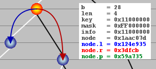
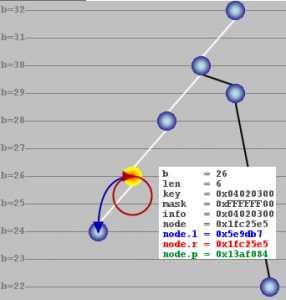
When the mouse is hovered over a node in the tree panel, the color of the node changes to orange and node information is displayed as follows:

Detail view of PATRICIA tree node
In the example screenshot above, the selected node is inserted for bit position 28. Len is the distance, i.e. number of bit positions, from the head node (4 in the screenshot above). The key for the node is 0×11000000 while the mask (network mask for IP address) is 0xFF000000. The search information stored in the node is 0×11000000 (info field). The pointers node.l and node.r point to other nodes depending on the PATRICIA algorithm. Finally, node.p points to the parent node.
How the search works
When the search animation starts, either all keys in the route file or the single key in the key field are searched for. The tree iterates through the nodes of the tree, starting at the head node (bit position b=32).
The search wanders down the tree starting at the head node moving towards the leave nodes. The search algorithm compares the bit of the search key at each encountered node’s bit position with the corresponding bit in the node’s key. If they are both 1, the algorithm navigates to the node referenced by node.r (“right” pointer), otherwise the search continues with the node pointed to by node.l (“left” pointer). The beauty of PATRICIA lies in the fact that only a limited number of nodes need to be traversed, in contrast to fully populated binary trees that have a node at each bit position.
When the search arrives at a leaf node (both node.l and node.r point to either the node itself or to nodes with bit positions higher up in the tree towards the head node), the search key is compared to the leaf node’s key (full match comparison, i.e. all bits are compared for equality). If both keys equal, the search was successful and the found target (info) is displayed right to the node with the node’s appearance changed to inverted orange:
Successful key search
So far, things were pretty standard PATRICIA algorithm. In Internet Protocol routing lookups, the netmask defines the bits that are compared in an IP address (search key) and a route table’s route prefix (node’s key). Even though non-contiguous netmask bits are possible in IP routing (and supported by this PATRICIA simulator), it is customary (and wise) to use contiguous netmasks starting at tradedoubler.com the left side (high order bits).
When the search hits a leaf node, the bits used for comparison of the search key and the node’s key are defined by the mask. When the comparison shows equality, the search was successful and the info (target) is displayed. When the comparison fails, the search backs up towards the root following the node.p (parent) pointers and performing a full match comparison using the mask in each node.
This behavior shows how a route lookup in IP routing works (IP forwarding is the correct term as routing means the protocols used to exchange IP routes between routers). Even though a specific route entry may match a given IP address using the netmask, there may be a better route where more bits match (a more specific route). The longest prefix match is what a route lookup should yield. The PATRICIA algorithm enhanced with evaluating netmasks is a practical algorithm to achieve this in software.
Structure of the route file
The PATRICIA simulator comes with 5 built-in route files:
| RouteFile_large.txt |
Large route file with 88 route entries and default route |
| RouteFile_small.txt |
Small route file with 18 route entries and default route |
| RouteFile_minimal.txt |
Very small route file with 8 route entries and default route |
| RouteFile_shallow.txt |
Route file with few routes resulting in a small and shallow PATRICIA tree |
| RouteFile_noDefaultRoute.txt |
Very small route file with 8 route entries but no default route |
The route files used by this PATRICIA simulator contain route entries on each line as follows:
# Key       Mask        Info
0x7f000001, 0xffffffff, 0x7f000001
0x11000000, 0xff000000, 0x11000000
Key, mask and info are separated by commas. Lines that start with a hash sign (#) are comment lines. These lines are ignored by the PATRICIA simulator. The Key entry corresponds to an IP address to be looked up, Mask corresponds to the netmask defining the prefix length and Info is the target of the lookup (in a real IP router this would be the interface over which to forward the IP packet). For the sake of simplicity, Info equals the key in the built-in route files.
A final word on default routes. A default route is identified with key=0×00000000 (IP address does not matter) and mask=0×00000000 (no bits are compared thus every IP address looked up matches). When such a default route is present in the route file, it is added to the head node. When an inexistent key (IP address) is input to the search algorithm, there will be no match in any of the tree’s nodes, so after having reached a leaf node, the search will back up towards the root of the tree (head) where there will be a match due to the default route (both key and the node’s key masked with 0×00000000 and compared to equality will match because all bits are masked out). So the default route is a route of last resort (matches if no other route matches). It is the last route to use because it has the shortest prefix length of all routes (zero bits).
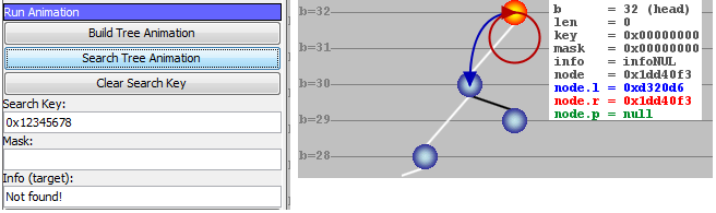
This behavior can be demonstrated by loading e.g. RouteFile_minimal.txt. Search for a key (IP address) that none of the routes in the loaded route file matches (simply enter the key=IP address in the control panel’s Search Key field in hexadecimal format such as 0xCAFE1234 and press Search Key Animation). The search will only yield a match in the head node (bit index b=32) where the default route resides. Now load RouteFile_noDefaultRoute.txt which does not contain a default route. Again search for a non-matching key. The search will fail because there is no longest-prefix match in any of the tree nodes and no default route that would normally match in the head node. The search failure is shown as follows:
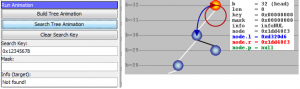
Failed search for a key (IP address)
The search failure is indicated with “Not found!” in the Info (target) field in the control panel. Additionally, the information that is displayed for the head node shows info=infoNUL.
Wrap up
PATRICIA tree simulator is a simple Java-based GUI tool for demonstrating the PATRICIA algorithm for IP route lookups. The algorithm is enhanced with functions to evaluate the netmask as well (longest-prefix match). The key, mask and info length are all 32 bits in length as is the case for IPv4 addresses. With some minor modifications, the simulator would work with 128 bit keys as well thus mimicking IPv6 addresses.